Week 1 — Training My First Classification Model

Introduction

I’ve started a structured journey into applied AI and machine learning.

My background is in building large-scale fintech and payment platforms. Increasingly, many of the most interesting problems in these systems are not purely infrastructure problems — they are decision problems. Fraud detection, anomaly detection, and intelligent risk systems all depend on models that learn patterns from data.

To understand these systems properly, I’m working through machine learning from first principles and documenting the process publicly.

This first experiment focuses on the basic structure of a supervised machine learning problem.

The building blocks

Every supervised learning system begins with three components.

Dataset
A collection of examples.

Features
The input values describing each example.

Label
The correct outcome we want the model to predict.

In a payments context, features might include transaction amount, merchant category, or device type, while the label might simply be fraud or not fraud.

The model’s task is to learn patterns that relate the features to the label.

The experiment

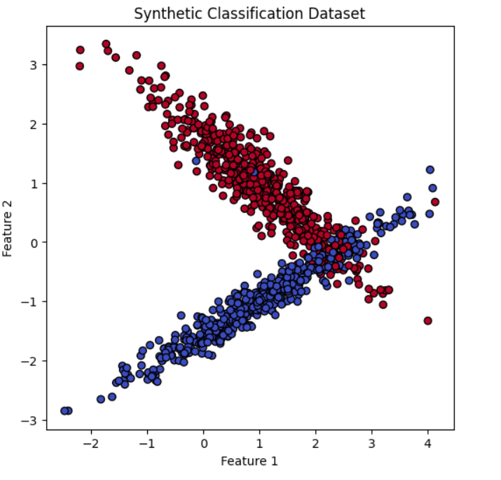
For this experiment I generated a synthetic dataset using scikit-learn.

The dataset contained:

• 1000 examples
• 2 features per example
• a binary label (class 0 or class 1)

Synthetic datasets allow the mechanics of machine learning to be explored without needing to build a real-world data pipeline first.

Train/test split

Before training a model, the dataset is divided into two parts.

Training data teaches the model the relationship between features and labels.
Test data evaluates how well the model performs on unseen examples.

In this experiment:

• Training examples: 800
• Test examples: 200

This separation helps ensure that the model is evaluated fairly rather than simply memorizing the training data.

The model

I trained a Logistic Regression classifier, a classical machine learning algorithm that learns a decision boundary separating two classes in feature space.

Despite its simplicity, logistic regression is still widely used in production systems and provides a clear introduction to classification.

Result

The model achieved:

Accuracy: 0.90

This means the classifier correctly predicted roughly 180 out of 200 unseen examples in the test set.

Because the dataset was balanced between the two classes, accuracy is a reasonable first performance metric.

Visualising the decision boundary

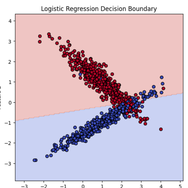
Because the dataset had only two features, it was possible to visualise both the data points and the classifier’s decision boundary.

This made the model much easier to understand.

Rather than treating machine learning as abstract statistics, the experiment made it visible: the classifier was effectively learning a line that separates two regions of feature space.

That geometric view made logistic regression feel much more intuitive.

Key takeaway

The most important outcome of this experiment is understanding the structure of the machine learning workflow:

1. inspect the dataset
2. split training and test data
3. train a model
4. generate predictions
5. evaluate performance

Nearly every applied machine learning system follows some variation of this pipeline.

What comes next

Future experiments will explore topics that become critical in real-world systems:

• imbalanced datasets
• confusion matrices
• precision and recall
• why accuracy alone can be misleading

These concepts are especially important in domains such as fraud detection where the events of interest are rare.

Code

Experiment notebook:
AI-Learning-Lab on GitHub